•Setup: When the setup for WallsMap is run, the executable (WallsMap.exe) is copied to whichever application folder you select. Also two file associations are set up: WallsMap project files (layerset files) have extension NTL while WallsMap-specific image files have extension NTI. Later you may want to also associate the SHP extension with WallsMap using the Open With dialog in Windows Explorer.
•Open Sample: Normally setup will finish by creating a program link on your desktop and automatically opening a sample project. Also, by default, whenever you run the program it will open the last loaded project file and present a map view covering all visible layers. The Preferences menu offers options for specifying whether or not the last project opens automatically, and, for an open project, whether or not the last view extent is restored each time it's opened.
•Open Layers Window: To see what image files and shapefiles exist as layers, open the Layers/Properties window by clicking on a toolbar icon as shown here:
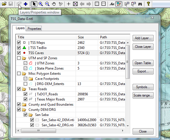
This window is resizable and can optionally stay open and serve as a legend as you browse the map. You can use the window for adding, deleting, and rearranging layers (by left-dragging with the mouse), and for toggling their visibility via the checkboxes. The rendering order for map display is from the bottom of the list to the top, meaning that imagery for a layer can obscure that of any layers beneath it.
When a layer is highlighted (see TSS Caves above), two buttons on the right panel open dialogs for fine tuning how the layer's information is processed. A Symbols dialog lets you specify colors and shapes for lines and symbols, labeling options, and other settings affecting the layer's appearance. For point shapefiles you can also specify, in the same dialog, which attribute fields are searched by default for selection purposes. For all layers you can limit their display and/or labeling to a specific Scale range. (See Setting Display Attributes.)
When a raster image layer is highlighted, the Symbols button is relabeled Opacity. It opens the Raster Image Opacity dialog for specifying how transparent the layer should be when rendered. In the above example a Digital Elevation Model (DEM) image is assigned an opacity of 30%, causing it to produce a 3D effect for the topographic map image (DRG) immediately below it in the layer sequence. (The DEM also supplies elevation information for the program.)
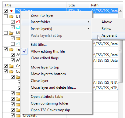
If map layers are grouped into folders and subfolders, you can expand or collapse tree branches by double-clicking. By using folders we simplify the displayed list of layers, making it much easier to control the visibility of groups of related files. Also, scale range settings can be quickly applied to an entire branch. You'll find options for creating folders in the right-click context menu for a selected tree item. Up to 8 levels of depth are supported.
The visibility of layers within a tree branch depends on their own checked status as well as that of their parent folders. A bold checkmark indicates that the layer will display when the map's scale is in the allowable range. For point shapefiles, a bold checkmark also indicates they are available for selection by text search assuming you haven't disabled them for text searches in the Symbols dialog for point features.
•Examine Different Layer Types: The top several layers in the above example have colored symbols next to their checkboxes that identify them as shapefiles, the most widely-supported vector format for GIS. Typically you'll find point shapefiles, polygon shapefiles, and polyline shapefiles, the last two having their own characteristic symbol shape. Farther down in the tree you'll find georeferenced raster image files, which have associated (often embedded) information allowing them to be positioned accurately on a map.
Each shapefile is actually a set of at least three file components with the same base name but with specific extensions: a .SHP component containing the geometry (sets of points with geographical coordinates representing a feature), a .SHX component providing indexed access to the SHP, and a .DBF component storing a table of feature attributes that users can examine or edit. According to ESRI's shapefile technical description, the DBF component is a standard dBase file (evidently dBase-III), with an unspecified number of fields and with no restrictions on field type. Many programs are able to open it, including Microsoft Access.
Besides these required components, a shapefile might also have a projection file with extension .PRJ identifying the coordinate system, a .DBT component (required if memo fields are present), and possibly some components that are application specific. For example, this program will look for an optional .TMPSHP component containing field descriptions, editing requirements (such as alternative values to appear in drop-down lists), and instructions for initializing fields in new records. (See Template File Format.) It can also create a .DBE component, convenient for selecting edited features for review.
When you browse a folder for a layer to add, you'll normally see just the .SHP file names listed, along with all supported raster image files. You needn't be concerned about the other shapefile components except when transporting or backing up your project.
•Download Raster Images: The supported raster image types include GeoTIFF (.TIFF and .TIF), JPEG (.JPG), JPEG2000 (.JP2, .J2K, and .JPC), Enhanced Compressed Wavelet (.ECW), MrSID (.SID) and files with extensions .PNM, .PPM, .BMP, .GIF, and .PNG. There are dozens of additional GIS formats supported by the Geospatial Data Abstraction Library (GDAL) the program uses, but not all are enabled. Finally, there is a raster format with extension .NTI that's specific to WallsMap. Note that files with these extensions are most often not georeferenced, in which case the program behaves like an image viewer and opens them in separate, non-layered document windows. As with type SHP, you may find it useful to associate some of these image types with WallsMap. (To do this, right-click the file name in Windows Explorer, select "Open width..." from the context menu, and select WallsMap as the "program to open this kind of file.")
See Available Background Imagery for a list of NTI files you can download and use as backgrounds in Texas projects.
•Explore the Map: Use the toolbar controls or the right-click context menu to zoom and pan the map view. The mouse scroll wheel is convenient for zooming in and out, and there's a preference setting to control the type of zoom (same as in Google Maps by default). You can double-click inside a map window to toggle between the arrow cursor, which allows drag-box zooming, and the hand cursor, which allows panning. You can also zoom to specific resolutions via the right-click context menu. More conventionally, you can zoom via the toolbar buttons labeled "+" and "-", but I find this less convenient than the other methods.
Note that map views of georeferenced data will have a scale bar. Right click on the scale bar to toggle between types of units:
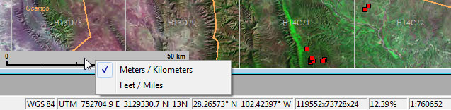
Also shown above is the program's status line, which normally displays information about the mouse pointer's geographical location (geodetic datum and both UTM and lat/long coordinates when known), the dimensions and color-depth of the topmost image at that location, the percent zoom for that image (at 100%, 1 screen pixel equals 1 image pixel), and finally the map's scale assuming your screen resolution is 96 dots-per-inch. If there is elevation data at that location, an elevation in feet or meters will replace the image dimensions.
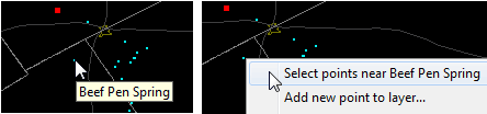
•Select Features by Location: To view or edit the attributes of point features shown on the map, right-click on a plotted symbol and choose Select points near... from the context menu.
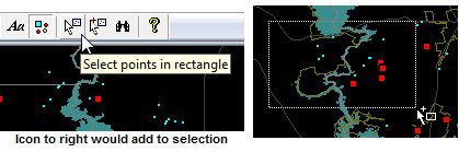
Alternatively, to select all features in a rectangular area on the map, click the toolbar icon with small white arrow and drag open a rectangle. (You can double-click to restore the arrow cursor.)
•Select Features by Attribute Value: A second way to select features is by searching specified attribute fields for text. Clicking the binocular toolbar icon opens a Text Search Operations dialog with some often-needed option settings, such as restricting the search to the map window's current extent. The dialog's find box also has a list of recently searched-for text items. Settings in this dialog won't affect searches via the find box at the bottom of the Selected Points window (see below). Searches done from there are not case sensitive, and they only examine the particular attribute fields set as searchable by default for the visible shapefile layers.
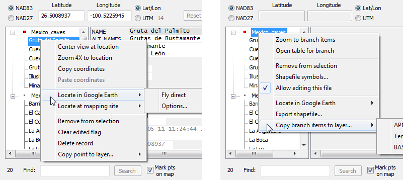
•Examine Attributes of Selected Items: When you select features using any of these methods the resizable Selected Points window will immediately open if not already open. It allows you to edit or view both locations and attributes, and also perform operations via two right-click context menus. One menu is for a selected record (below left) and the other is for all records selected in a particular shapefile (below right):
The Selected Points window can stay open as you browse the map and perform other operations.
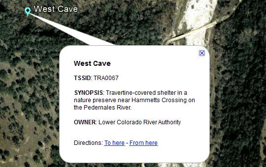
•View Multiple Point Features in Google Earth: Notice that in these menus, and also on other context menus (map view and table view), there's an option that launches Google Earth (GE) and puts one or more labeled placemarks on its map. If you choose Options instead of Fly direct from a submenu, the KML Options dialog lets you select the fields used for constructing the descriptions that appear when the GE user clicks on a placemark icon (example below). The icon size and style are also customizable. For more information about this feature, see Google Earth (KML) Launch Options.
• Center a Web Mapping Application at a Point: Another context menu choice is to open a web mapping application in your browser, centered on the point or feature you've chosen. This can be faster and more informative than using Google Earth when the goal is to inspect the roads, towns, and terrain surrounding a single generated placemark. A Preferences menu item named URL for Web Map Navigation lets you specify which application to open and what kind of map to initially display. The application that's set up by default is Acme Mapper. In addition to providing Google's standard map views, both it and a similar application, Gmap4, can display GIS data of several different kinds. It also has an interface that's convenient for grabbing coordinates for use in WallsMap, either for establishing new features or for placing persistent marks on the map view (see next item). Only a single copy/paste operation is needed.
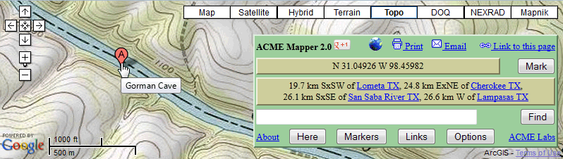
•Center the Map or Capture Coordinates: An operation you'll likely perform often is navigating to a specific location on your map using a set of coordinates you've copied to the Windows clipboard from some source. For example, it could be the set N 31.04926 W 98.45982 shown above, or some other format the program recognizes, such as N 31 2' 57" W 98 27' 35". Open the Center View on Point dialog by either clicking a toolbar button (crosshair icon) or by right-clicking a point on the map and selecting that option from the context menu:
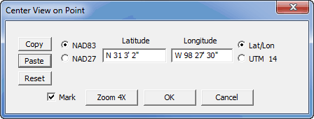
When there's a recognizable coordinate pair on the clipboard, the Paste button will be enabled. The coordinate boxes will be initialized to either the position clicked on or the previous centered-on position if access was via the toolbar. A cross-shaped placemark is optionally produced that remains in place until the next centering operation. As in the Selected Points dialog, which also supports copy/paste operations with coordinate pairs, you can convert between coordinate systems.
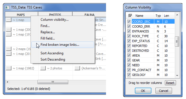
•Open a Table View: Currently, only point features are selectable via the map, and only 2D point shapefiles have editable geometry (locations). You can, however, open a spreadsheet view of the attributes of any shapefile and perform spreadsheet-style edits. The normal way to do this is by selecting the layer in the Layers/Properties window and clicking the Open Table button. Alternatively, to open the table for a selected subset of records, right-click a shapefile title in the Selected Points dialog and choose Open table for branch. You can then perform a variety of operations on the table, among them sorting on columns and selecting record subsets for export, possibly with specific columns hidden or rearranged. Be sure to try out the two pop-up context menus, one by right-clicking the table's header and another by right-clicking a selected row as shown here:
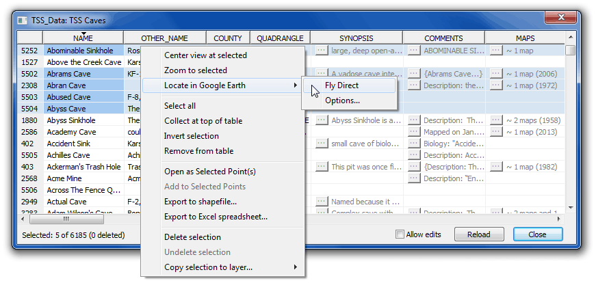
Note in particular the four export functions. You can generate a KML file for the selected records and fly directly to them with Google Earth. (The "Locate at mapping site" option isn't shown when more than one point is selected.) Similarly, you can export a new shapefile while specifying various options as described in Exporting and Merging. That topic also describes the Copy selection to layer function, which allows you to copy records to another loaded shapefile, even when their attribute structures aren't identical. Finally, the Export to Excel spreadsheet function creates an XLS file and optionally opens it with Microsoft Excel (or the associated program).
The table header's context menu offers fill and replace functions, a test for broken links in memo fields, and a quick way to rearrange or hide columns (apart from direct dragging), which can be useful when exporting either shapefiles or spreadsheets:
You'll find that it's possible to have both the Selected Points window and several table views open at once, perhaps displaying the same editable data. Records loaded in Selected Points are shown with a yellow tint in the table, with the specific record selected also grayed. At the same time, the map view is navigable and will display any information that's been committed. A pending new point will also be shown on the map.
•View Rich Text and Linked Image Files: All you'll find in the attribute tables of typical shapefiles are fixed-length fields not exceeding 255 characters in length. I believe that's simply because Esri has never supported memo fields in their GIS software. (Memos are a valid dBase-III field type and consistent with ESRI's shapefile technical description.) A memo field doesn't actually store its data in the DBF file component. It instead stores a 10-digit pointer to a set of contiguous 512-byte blocks of data in a separate DBT component. (See dBase format.) At least for us, this almost unlimited field capacity allows shapefiles to serve as the file format for a lightweight geodatabase.
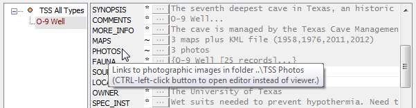
In table views and in the Selected Points window's right panel, memo fields appear as pushbuttons, with text alongside indicating the type of content. If the memo is non-empty and contains ordinary (ANSI) text, a leading portion of this text appears in gray to the button's right. If the memo instead contains rich text (RTF), the text fragment is enclosed in braces. In either case, clicking the button opens the program's text editor, one that supports both kinds of text. Active internet and local file links can be embedded in the text.
There's one exception to this behavior. If ordinary text is formatted a special way, the program interprets the text as a set of image links. In that case, clicking the button opens the program's image previewer, one that features a row of thumbnail images at the top of its window.
All three memo types are represented in the cluster of memos shown below. (Out of view are text, numeric, and logical fields whose fixed sizes are indicated by a white background.)
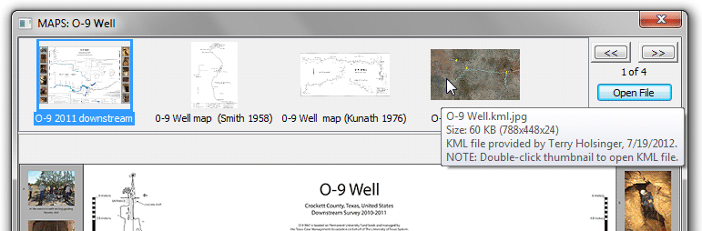
In this example, when you click on the MAPS button the image preview window shown below appears (or is refreshed):
Normally you won't need to manually edit the image links. (The format is easy to deduce by CTRL-clicking the button and viewing the text.) After you open an empty memo, a button labeled "Image Mode" on the text editor's frame will, when clicked, replace the editor window with the image preview window -- empty except for a banner that describes how to add images. Not mentioned is the fact that, in addition to drag-and-drop, you can cut-and-paste files from Windows Explorer. WallsMap stores relative pathnames in the memo field whenever possible -- relative, that is, to the folder containing the shapefile. This allows the project to be easily transported as long as the image folders are included. (Internet links are not yet supported by the image previewer.)
Be sure to examine the thumbnail panel's context menu. There are options for revising the thumbnail caption and entering additional text to appear in pop-up windows, such as photo credits. You can also enter a collection title that will appear to the right of the memo's button. Another option I use often is "Open containing folder", which positions Windows Explorer at the particular file.
The image preview itself, below the thumbnails, can't be zoomed or panned. It simply resizes to fit the resizable window while not exceeding the image's actual pixel dimensions. To examine large images in greater detail you can click the Open File button (or double-click the thumbnail). The program will then open the file as a separate document. You might not notice it at first since it will likely be partially obscured by the preview window.
The image previewer generates thumbnails on the fly. If the original file is very large or of a type not natively supported by WallsMap, you can use a feature that's illustrated in the above example. The approach is to create a different file to actually preview, a raster image with the same name as the original file but with the true extension tacked on at the end. In this example we've loaded a KML file named O-9 Well.kml in Google Earth, took a screenshot and saved it alongside the KML file as O-9 Well.kml.jpg. When the thumbnail for the image file is double-clicked, WallsMap recognizes the double extension and opens the KML in Google Earth, the associated application. This feature works well with PDF documents and video files where the user is likely to have a default viewer. (At least for now, the associated application is irrelevant if the original file is a supported image format. In that case it's opened as a separate document within the same instance of WallsMap.)
One more feature of the previewer is worth noting. If you choose to open a raster image that's georeferenced and compatible with the project, you're asked if it should be added as a layer (and/or zoomed to) instead of opened as a separate document.
•Generating NTI Files for Efficient Viewing: When you open a large graphics file (TIFF, SID, etc.) with the intention of examining it often, you should convert it to the WallsMap-specific NTI format. You can access the NTI export dialog via either the file menu (for a stand-alone file) or the "Export" button in the Layers window when the layer is highlighted. This is an easy, normally quick operation that will result in less memory usage, higher quality display in some cases, and much faster performance due to the presence lower-resolution overviews. When converting aerial photography to NTI, you might try the JPEG2000 compression option at 5% or even 3%. It's unlikely you'll lose significant detail, particularly with SID and ECW files that are highly compressed to begin with. For topographic map images, which normally use a 256-color palette, I've found that WebP compression at quality 80 gives good results. (For paletted images, only the overviews are lossy compressed.) For more information, see Converting Images to NTI Format.
•Synchronized Viewing of Multiple Layer Sets: After opening two or more georeferenced images or NTL projects try this: Tile the document windows vertically (there's a toolbar icon for this), then right-click a window and select "Synchronize on Point" from the context menu. (See top image in Introduction for a view of three synchronized projects.) While synchronized projects can have different coordinate systems (projection and datum), the program is currently limited in that all image layers in a single project must have the same coordinate system. (Datums NAD83 and WGS84 are treated as if they were equivalent.) Unlike shapefile layers, raster image layers are not reprojected "on the fly" when they are added.