Introduction
The sample Texas project contains a layered set of shapefiles, but no raster image layers. You can use it in that condition, selecting individual points and launching Google Earth/Maps to explore the surrounding topography, towns, and roads. With the addition of image layers, however, you'll be able to view all your shapefile data against a background that's faster to display and possibly of higher quality. Also, when inspecting aerial photography to retrieve coordinates for a feature, you'll likely get a more reliable result using a USGS Digital Orthophoto Quadrangle (DOQ) instead of Google's imagery. Google Earth's displayed coordinates, while typically accurate to within 6-10 meters, might be dozens of meters off. You can sometimes see this when examining GE imagery obtained in different years.
Like many GIS viewers, WallsMap imposes a restriction regarding raster imagery that's sometimes inconvenient: All raster files added to a single project must be georeferenced to the same coordinate system. That's because on-the-fly reprojection of raster data can't be implemented very efficiently. It can make more sense to convert the imagery you need just once, using other tools, rather than slow down the viewing process. Furthermore, at this stage in its development WallsMap recognizes only four combinations of geodetic datum and projection type: WGS84 (equivalently NAD83) or NAD27, and Lat/Long degrees or UTM meters. So images using other coordinate systems, such as Texas Sate Plane, have to be converted anyway.
Shapefiles are more flexibly handled since their geometry can be efficiently converted to the required coordinate system during the display process. For example, if the first image you add to the Texas project is a UTM zone 14 DOQ downloaded from TNRIS, the entire set of shapefiles will be displayed as if they had been reprojected to UTM zone 14. (The outline of Texas will immediately acquire a noticeably different shape.) Thereafter, if you wanted to add a Lat/Long image, you would need to remove any UTM images first. The program can provide the necessary prompts because coordinate system info is stored in the image file's header.
A possible workaround for this limitation is to select File | Save As to create a copy of the project file with a new name, then use it to display UTM imagery. That way you could add UTM DOQs to a functionally equivalent UTM Texas project. If not opened at the same time in different program instances, different projects can share the same set of shapefiles. Alternatively, if you have the right software tools (e.g., ArcGIS, Global Mapper, gdalwarp) you can reproject the imagery after downloading it.
TSS Resources
NTI Files Available for Texas Projects
Except where noted, the image data described here use the NAD83 (or WGS84) Lat/Long coordinate system and can be added directly to the Texas project as long as no image with a different projection is already present. Note that the exe files are self-extracting archives. You just need to execute each one while specifying a folder, such as Texas_NTI, to store the contained files. When you add one of the large NTI files to the project for the first time, you might be notified that a one-time expansion of file size is necessary. This process of adding lower-resolution "overviews" shouldn't take more than a couple of minutes. (To avoid this prompt with each such addition, you can download and extract all the archives first, then add the layers as a group -- for example, by selecting and dragging multiple NTI files from a Windows Explorer window to the Layers window of your open project.)
DEM and DRG Layers for the Texas Hill Country
This section lists downloadable image archives for 23 rectangular regions covering a total of 1177 USGS 7.5' quadrangles in Texas. You can choose which of these layers to download and add to your project, but the program's performance shouldn't suffer noticeably if you include them all. The self-extracting archives each contain a single NTI image made up of tiled topographic maps, Digital Raster Graphics (DRGs), along with a 1/3 arc-second Digital Elevation Model (DEM) layer covering the same region. The original image quality of the scanned USGS topos downloaded from TNRIS is preserved. (At full resolution the compression method is lossless).
The DEM layer is comprised of two files: an NTI image that you explicitly add to the project and an optional NTE file that the program will automatically access to retrieve elevations. When made partially transparent the NTI component can add an attractive 3D shading to an underlying topographic map image. (See screenshot below.) The NTE component, if present, allows elevations to be shown on the status line as you move the mouse cursor over its area of coverage. (You can choose feet or meter units for the display.) Another benefit is that elevation fields for new or relocated shapefile records are automatically initialized if that option was specified in the shapefile's template component. (See Location-dependent Initialization.) The availability of elevations won't depend on the DEM layer's visibility setting or its position in the Layers window; only its existence in the project is necessary. With a DEM present and the topos visible, for example, you can see how well the displayed elevations match the contour lines.
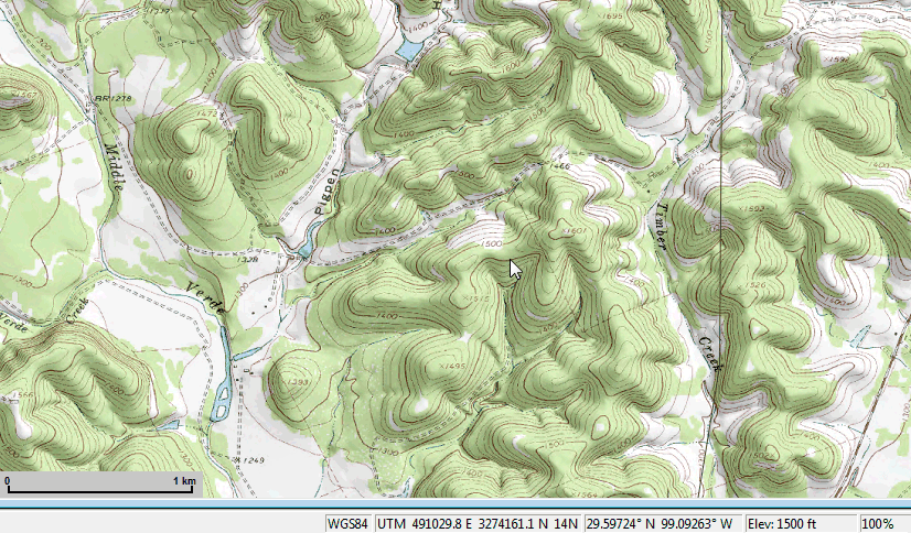
In the above screenshot the DEM layer is displayed with 30% opacity above a USGS topographic map (DRG) to provide a shaded effect. The 100% indicated on the status line, therefore, applies to the DEM layer's zoom level. The corresponding zoom level of the underlying DRG is about 38%.
The image below shows the locations of the 23 DEM/DRG datasets currently available for download. Each rectangular region is covered by two image layers as described above: a grayscale 1/3 arc-second DEM image (with associated NTE elevation file) and a DRG image consisting of tiled topographic maps.
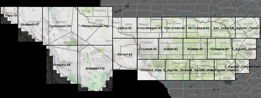
The datasets are self-extracting archives. If all are downloaded, they will occupy 10.7 GB of hard disk space when expanded. More than half of this, however, is claimed by the NTE files whose only role is to provide elevations for display on the status line and for dynamically initializing elevation fields. If you don't need these capabilities, simply delete the NTE file after it's extracted from a downloaded archive.
➢19 quads (El Paso)
El_Paso-19.exe (50 MB)
➢57 quads (Hudspeth)
Hudspeth-57.exe (150 MB)
➢110 quads (Culberson, N Jeff Davis)
Culberson-110.exe (290 MB)
➢69 quads (Presidio, S Jeff Davis)
Presidio-69.exe (229 MB)
➢110 quads (Loving, Pecos, Reeves, Ward, Winkler)
Pecos-Reeves-110.exe (205 MB)
➢118 quads (Brewster)
Brewster-118.exe (386 MB)
➢63 quads (Terrell, E Pecos )
Terrell-63.exe (210 MB)
➢42 quads (Upton, E Crane, N Pecos)
Upton-42.exe (83 MB)
➢42 quads (Reagan, W Irion, N Crocket)
Irion-Reagan-42.exe (90 MB)
➢42 quads (Tom Green, E Irion, N Schleicher)
Tom Green-42.exe (119 MB)
➢42 quads (Concho, McCulloch, N Menard)
McCulloch-42.exe (126 MB)
➢42 quads (San Saba, Mills, W Lampasas)
San_Saba-42.exe (135 MB)
➢42 quads (Bell, Coryell, E Lampasas)
E_Aquifer_Farnorth.exe (128 MB)
➢36 quads (Crockett, N Val Verde)
Crockett-36.exe (147 MB)
➢42 quads (Sutton, S Schleicher)
Sutton-42.exe (119 MB)
➢42 quads (Kimble, S Menard)
Kimble-42.exe (127 MB)
➢42 quads (Gillespie, Llano, W Blanco, E Mason)
Gillespie-42 (142 MB)
➢42 quads (Travis, N Hays, S Burnet, E Blanco, W Williamson)
E_Aquifer_North.exe (158 MB)
➢39 quads (S Val Verde)
Amistad_Area.exe (162 MB)
➢42 quads (S Edwards, N Kinney, W Real, NW Uvalde)
E_Aquifer_Farwest.exe (149 MB)
➢42 quads (Bandera, S Kerr, NW Medina, E Real, NE Uvalde)
E_Aquifer_West.exe (102 MB)
➢36 quads (E Bandera, N Bexar, S Blanco, W Comal, Kendall, NE Medina)
E_Aquifer_Central.exe (151 MB)
➢16 quads (E Comal, S Hays)
E_Aquifer_Central-East.exe (38 MB)
GE
Geologic Map Images with Associated Shapefiles
➢Geologic Atlas of Texas (GAT)
GAT_250K.nti (434 MB)
This image covers the entire state and was assembled from the 38 map sheets making up the Geologic Atlas of Texas (GAT). A convenient web interface for viewing the 1:250,000 scale maps, including margin information, is provided by the Texas Water Development Board. A polygon shapefile, with the GAT rock codes and other attributes, is contained in this self-extracting archive:
GAT_250K.exe (331 MB, or 607 MB after extraction).
By adding it as an invisible project layer, with spatial indexing enabled, you can set up a point shapefile to have a field dynamically initialized with codes like Ked that depend on a point's location. (See Location-dependent Initialization in the Template File Format topic.)
➢Maps from the Geologic Database of Texas (GDOT)
GDOT_(4_NTI-SHP_sets).exe (161 MB)
These four layer sets (NTI with corresponding shapefile) were derived from the Geologic Database of Texas, an Esri personal geodatabase available at the TNRIS website. In addition to the 1987-vintage GAT in vector form, the geodatabase contains several GIS databases published by the Texas Bureau of Economic Geology. The layers chosen for this archive cover four discontiguous regions, all but one mapped at scale 1:24,000.
•GDOT_Georgetown_1997-99: Most of the the western half of Williamson Co. and parts of adjacent counties (16 7.5' quadrangles).
•GDOT_Austin_2002: Central Travis County (about ten 7.5' quadrangles), mapped at scale 1:62,500.
•GDOT_NewBraunfels_1997: Northern Bexar Co., all of Comal Co., and all but the northern third of Kendall Co. (32 7.5' quadrangles).
•GDOT_DelRio_2001: An area surrounding Amistad Dam, Del Rio, and Laughlin AFB in Val Verde Co. (9 7.5' quadrangles).
As with the statewide GAT, these layers and the ones from USGS below can be used for automatic field initialization, with the GAT shapefile used as the fall-back. The NTI images, when present in a project, can be toggled on as needed to view the surrounding surface geology.
➢Geologic Maps and Shapefiles Derived from USGS Publications
USGS_Texas_Geology_(4_NTI-SHP_sets).exe (82.2 MB)
The PDF-derived NTI images and shapefiles in this archive incorporate data from recent USGS reports:
Map Showing Geology and Hydrostratigraphy of the Edwards Aquifer Catchment Area, Northern Bexar County, South-Central Texas
http://pubs.usgs.gov/of/2009/1008/
Geologic Map of the Edwards Aquifer Recharge Zone, South-Central Texas
http://pubs.usgs.gov/sim/2005/2873
Geologic Map of the Edwards Aquifer and Related Rocks in Northeastern Kinney and Southernmost Edwards Counties, South-Central Texas
http://pubs.usgs.gov/sim/3105/
Geologic Map of Big Bend National Park, Texas
http://pubs.usgs.gov/sim/3142/
Miscellaneous High-Resolution Imagery
➢Government Canyon State Natural Area
GCSNA_15cm_2010.nti (285 MB, expands to 409 MB when opened)
This 15-cm resolution aerial image covers a 7.5 km by 9 km rectangle in NW Bexar County. It was extracted using the USGS National Map Viewer, converted from UTM to a Lat/Long, and exported as an NTI file using 3% JPEG2000 compression. Metadata lists Jan 2010 as the acquisition date.
➢Spring Branch Area
Spring Branch_15cm_2010.nti (125 MB)
This image covers a 3 km by 4.5 km section of the Spring Branch karst area in Comal and Kendall counties. Its top-right edge is aligned with the northern boundary of the San Antonio area 0.15-m imagery acquired during Jan-May of 2010. (See map of boundary below.) Its top-left corner and far left edge (about 20%) had to be constructed from 1-meter imagery of the same time period.
➢Honey Creek State Natural Area
Honey Creek_15cm_2010.nti (212 MB, expands to 308 MB when opened)
Another 15-cm resolution image covering a 9 km by 6 km region on the border between Kendall and Comal counties. It encompasses the known extent of Honey Creek Cave, the longest cave in Texas.
➢Cedar Park Cave Area
CedarPark_15cm_2009.nti (151 MB)
This 5.5 km x 4.4 km area encompasses several cave preserves in southern Williamson County. The area contains numerous caves despite it being densely developed.
➢Lake Belton Area of Ft Hood
Ft_Hood_Lake_Belton.nti (346 MB, expands to 492 MB when opened)
This is an attractive 0.3-meter resolution aerial photo covering NW Ft Hood and most of Lake Belton.
➢Amistad Lake Area Landsat
Amistad_Lake_Area_Landsat.nti (2.4 MB)
This is a 26.8 meter/pixel, USGS Landsat image covering southern Val Verde County. It's of higher quality than the one for all of Texas (below) and shows a dramatically lower lake level.
➢Landsat 7 image of Texas
texas_landsat.nti (266 MB, expands to 377 MB when opened)
This image was created earlier than April 2006. It's an attractive background but perhaps less useful now that more recent and higher quality imagery can be easily accessed via Google Earth and web mapping sites using the program's "fly to" feature. Like the other files in this section, it would need to be removed prior to adding a downloaded UTM image.
Online Resources
TNRIS - Texas Natural Resources Information System
From the TNRIS Data Search and Download page you can select a county or quadrangle and download any of several types of georeferenced images. Among them are 1-meter resolution Digital Orthophoto Quarter Quads (DOQQs) from the National Agriculture Imagery Program (NAIP). The latest version of this imagery, dated 2010, is provided in two formats. The better-quality version uses the JPEG2000 format (extension JP2) and covers the standard DOQQ area, which is 1/4 of a USGS 7.5' quadrangle. The same imagery is also available in the form of Compressed County Mosaics (CCMs), which are very large Multi-resolution Seamless Image Database (MrSID) images (extension SID) covering an entire county. I don't recommend the latter because of their size (typically more than a gigabyte), fewer colors, and lower overall quality. The CCMs are compressed 15:1 whereas the individual DOQQs are compressed 5:1. (The TNRIS site states that uncompressed GeoTIFF DOQQs are available by special request.)
Another DOQQ choice worth considering are half-meter resolution photos obtained in Sept 2008, with each zip archive containing both a 3-band Natural Color (NC) JP2 file and a 3-band Color Infrared (CIR) JP2 file. A sample of the NC version is shown at the bottom of this page. All DOQQs at TNRIS are projected to UTM (NAD83) and can be read directly by WallsMap.
Two versions of scanned USGS 7.5' topos, with their collars trimmed, are also available at the same download page. Unfortunately, neither would be compatible with any Lat/Long NAD83 image layers in a WallsMap project. That's because one version is Lat/Long NAD27 (same as the paper original) and the other version is UTM NAD83. To produce the DEM/DRG images, I used Global Mapper to assemble and reproject a grid of NAD27 quads to produce a seamless Lat/Long, NAD83 geoTIFF. I then used WallsMap to create an NTI image. (The JPEG2000 method at 10% compression ratio was chosen for each NTI export, but since the USGS topos are 256-color images, the program uses lossy compression only for the overviews. There is no quality loss at zoom levels greater than 50%.)
USGS - United States Geological Survey
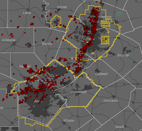
The USGS National Map web page introduces the National Map Viewer, an interactive web application that supports the direct download of various kinds of GIS files. (This application replaces the Seamless Server, which was retired on July 31, 2012.) For example, you can download the 15-cm resolution orthoimagery that's available for certain regions of Texas. The yellow outlines in the image below show several such regions in early 2011, with red dots indicating Texas Speleological Survey cave locations. For the San Antonio region, the most recent 15-cm data was acquired in 2010. I found that when you use the viewer to select an area for obtaining 15-cm imagery you'll be emailed links to a set of zip files. Each zip, about 250 MB in size, will store an uncompressed geoTIFF covering a 1500 m x 1500 m region. The file will be georeferenced UTM zone 14, NAD83.
The National Map Viewer also provides access to a 70-km wide band of 0.3-meter orthoimagery covering the US-Mexico border. It extends about 45 km into Texas and is perhaps the best imagery available for this region, which includes the areas surrounding Lake Amistad. In the places I've checked, this UTM imagery is of much higher quality than what you can currently see in Google Earth.
Another important data type available for download are 1/3 arc-second National Elevation Dataset (NED) files in ArcGrid format. Each zip is about about 360 MB in size and contains data covering a square degree. The data must be converted to NTI / NTE file sets before they can be used in WallsMap for elevation retrieval and 3D shading. (I haven't documented the conversion method, but will soon.) 1/9 arc-second NED files are also becoming available for parts of Texas.
The USGS is also offering topographic maps at the National Map - US Topo website. Both old and new topo editions are being provided as GeoPDFs, with the latest releases being in vector format. Unfortunately, much of the interesting detail found on the older topo sheets (minor contours, houses, names of steams, canyons, etc.) is missing from the vector versions, which were designed to be viewed superimposed on an orthoimage layer in the PDF. The good news is that while the GeoPDFs containing the older editions don’t have an orthoimage, the several that I've downloaded have high-resolution scans of the original topo sheet. The pixel resolution of a 7.5' topo image obtained at TNRIS, for example, is 5259 x 5259. The scan of that same sheet in the GeoPDF has a resolution of 13695 x 13695.
CAPCOG - Capital Area Council of Governments
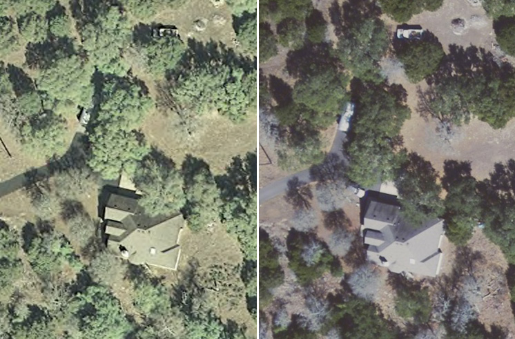
At CAPCOG's Geospatial Data page, you can download a variety of shapefile and image data for ten Texas counties: Bastrop, Blanco, Burnet, Caldwell, Fayette, Hays, Lee, Llano, Travis, and Williamson. Both the shapefiles and images at CAPCOG have to be converted from State Plane (Texas Central Zone) to either UTM or Lat/Long for use in the Texas WallsMap project. Also, when I last checked the site, the best available imagery was in the form of lossy-compressed MrSID files.
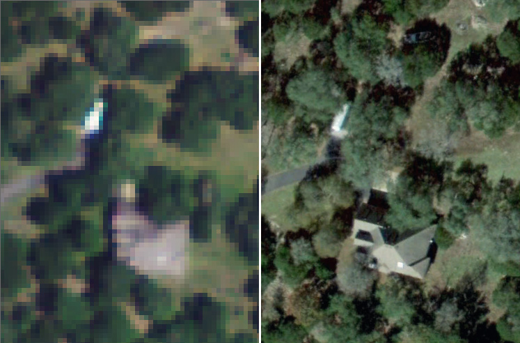
Below is a typical 60 m x 75 m aerial view, with CAPCOG's 2009 6-in imagery (top-left) alongside USGS 2006 6-in imagery for the Austin area (top-right). Note that CAPCOG's MrSID file contains artifacts from lossy compression whereas the USGS TIFF file is uncompressed and has a better color range. (Both are shown at 100% zoom.) The bottom two images show the 0.50-meter DOQQ available at TNRIS (left) and Google Earth imagery dated Nov 2009 (right). This comparison was done with imagery obtained in early 2011.